Introducción
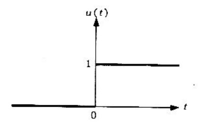
La función escalón unitario está definido como
Después, se va a suponer que
Se recuerda que
Donde
Por lo que
excpeto cuando
Ahora, se agrega una nueva suposición
donde
Se recuerda que
de donde se concluye que
Para encontrar
Como
Regresando
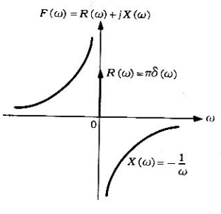
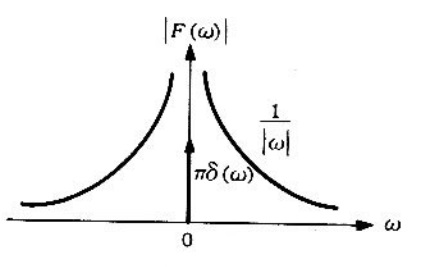
Figura 1. Función escalón unitario. Figura 2. Transformada de Fourier de la función escalón unitario. Figura 3. Espectro de la función escalón unitario. La función signum
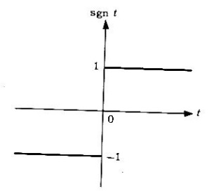
Sea signum y está definido como
Como la función
Ahora, se sabe que
Continuando
Donde
Figura 4. Función sgn t Figura 5. Espectro de la función sgn t Teorema
Teorema 1. Como
debido a que
Entonces, si
Publicado por Cesar Reyes
Dedicado a compartir información temas referentes al cálculo básicos, intermedios y avanzados mediante presentaciones PDF, videos y publicaciones en este sitio web.
Ver todas las entradas de Cesar Reyes

![\displaystyle \mathcal{F} [u(t)] = F(\omega)](https://s0.wp.com/latex.php?latex=%5Cdisplaystyle+%5Cmathcal%7BF%7D+%5Bu%28t%29%5D+%3D+F%28%5Comega%29&bg=ffffff&fg=192930&s=0&c=20201002)
![\mathcal{F}[f(-t)] = F(-\omega)](https://s0.wp.com/latex.php?latex=%5Cmathcal%7BF%7D%5Bf%28-t%29%5D+%3D+F%28-%5Comega%29&bg=ffffff&fg=192930&s=0&c=20201002)
![\displaystyle \mathcal{F}[u(-t)] = F(-\omega)](https://s0.wp.com/latex.php?latex=%5Cdisplaystyle+%5Cmathcal%7BF%7D%5Bu%28-t%29%5D+%3D+F%28-%5Comega%29&bg=ffffff&fg=192930&s=0&c=20201002)


![\mathcal{F}[u(t)] + \mathcal{F}[u(-t)] = \mathcal{F}[1]](https://s0.wp.com/latex.php?latex=%5Cmathcal%7BF%7D%5Bu%28t%29%5D+%2B+%5Cmathcal%7BF%7D%5Bu%28-t%29%5D+%3D+%5Cmathcal%7BF%7D%5B1%5D&bg=ffffff&fg=192930&s=0&c=20201002)


![\displaystyle \mathcal{F}[u'(t)] = \mathcal{F}[\delta(t)]](https://s0.wp.com/latex.php?latex=%5Cdisplaystyle+%5Cmathcal%7BF%7D%5Bu%27%28t%29%5D+%3D+%5Cmathcal%7BF%7D%5B%5Cdelta%28t%29%5D&bg=ffffff&fg=192930&s=0&c=20201002)

![\displaystyle j \omega [\pi \delta(\omega) + B(\omega)] = 1](https://s0.wp.com/latex.php?latex=%5Cdisplaystyle+j+%5Comega+%5B%5Cpi+%5Cdelta%28%5Comega%29+%2B+B%28%5Comega%29%5D+%3D+1&bg=ffffff&fg=192930&s=0&c=20201002)


![\displaystyle \mathcal{F}[u(t)] = F(\omega)](https://s0.wp.com/latex.php?latex=%5Cdisplaystyle+%5Cmathcal%7BF%7D%5Bu%28t%29%5D+%3D+F%28%5Comega%29&bg=ffffff&fg=192930&s=0&c=20201002)
![\displaystyle \mathcal{F}[u(t)] = k \delta(\omega) + B(\omega)](https://s0.wp.com/latex.php?latex=%5Cdisplaystyle+%5Cmathcal%7BF%7D%5Bu%28t%29%5D+%3D+k+%5Cdelta%28%5Comega%29+%2B+B%28%5Comega%29&bg=ffffff&fg=192930&s=0&c=20201002)
![\displaystyle \therefore \mathcal{F}[u(t)] = \pi \delta(\omega) + \frac{1}{j\omega}](https://s0.wp.com/latex.php?latex=%5Cdisplaystyle+%5Ctherefore+%5Cmathcal%7BF%7D%5Bu%28t%29%5D+%3D+%5Cpi+%5Cdelta%28%5Comega%29+%2B+%5Cfrac%7B1%7D%7Bj%5Comega%7D&bg=ffffff&fg=192930&s=0&c=20201002)

![\displaystyle \mathcal{F}[\text{sgn} \, t] = F(\omega)](https://s0.wp.com/latex.php?latex=%5Cdisplaystyle+%5Cmathcal%7BF%7D%5B%5Ctext%7Bsgn%7D+%5C%2C+t%5D+%3D+F%28%5Comega%29&bg=ffffff&fg=192930&s=0&c=20201002)


![\displaystyle \mathcal{F}[f'(t)] = \mathcal{F}[2 \delta(t)]](https://s0.wp.com/latex.php?latex=%5Cdisplaystyle+%5Cmathcal%7BF%7D%5Bf%27%28t%29%5D+%3D%C2%A0%5Cmathcal%7BF%7D%5B2+%5Cdelta%28t%29%5D&bg=ffffff&fg=192930&s=0&c=20201002)


![\displaystyle \mathcal{F}[\text{sgn} \, t] = \frac{2}{j\omega}](https://s0.wp.com/latex.php?latex=%5Cdisplaystyle+%5Cmathcal%7BF%7D%5B%5Ctext%7Bsgn%7D+%5C%2C+t%5D+%3D+%5Cfrac%7B2%7D%7Bj%5Comega%7D&bg=ffffff&fg=192930&s=0&c=20201002)
![\displaystyle \text{sgn} \, t = \mathcal{F}^{-1} \left[\frac{2}{j\omega} \right]](https://s0.wp.com/latex.php?latex=%5Cdisplaystyle+%5Ctext%7Bsgn%7D+%5C%2C+t+%3D+%5Cmathcal%7BF%7D%5E%7B-1%7D+%5Cleft%5B%5Cfrac%7B2%7D%7Bj%5Comega%7D+%5Cright%5D&bg=ffffff&fg=192930&s=0&c=20201002)
![\displaystyle \text{sgn} \, t = 2 \mathcal{F}^{-1} \left[\frac{1}{j\omega} \right]](https://s0.wp.com/latex.php?latex=%5Cdisplaystyle+%5Ctext%7Bsgn%7D+%5C%2C+t+%3D+2+%5Cmathcal%7BF%7D%5E%7B-1%7D+%5Cleft%5B%5Cfrac%7B1%7D%7Bj%5Comega%7D+%5Cright%5D&bg=ffffff&fg=192930&s=0&c=20201002)
![\displaystyle \frac{1}{2} \text{sgn} \, t = \mathcal{F}^{-1} \left[\frac{1}{j\omega} \right]](https://s0.wp.com/latex.php?latex=%5Cdisplaystyle+%5Cfrac%7B1%7D%7B2%7D+%5Ctext%7Bsgn%7D+%5C%2C+t+%3D+%5Cmathcal%7BF%7D%5E%7B-1%7D+%5Cleft%5B%5Cfrac%7B1%7D%7Bj%5Comega%7D+%5Cright%5D&bg=ffffff&fg=192930&s=0&c=20201002)
![\displaystyle \therefore \mathcal{F}^{-1} \left[\frac{1}{j\omega} \right] = \frac{1}{2} \text{sgn} \, t](https://s0.wp.com/latex.php?latex=%5Cdisplaystyle+%5Ctherefore+%5Cmathcal%7BF%7D%5E%7B-1%7D+%5Cleft%5B%5Cfrac%7B1%7D%7Bj%5Comega%7D+%5Cright%5D+%3D+%5Cfrac%7B1%7D%7B2%7D+%5Ctext%7Bsgn%7D+%5C%2C+t&bg=ffffff&fg=192930&s=0&c=20201002)

![\mathcal{F} [f(t)] = F(\omega)](https://s0.wp.com/latex.php?latex=%5Cmathcal%7BF%7D+%5Bf%28t%29%5D+%3D+F%28%5Comega%29&bg=ffffff&fg=192930&s=0&c=20201002)
![\displaystyle \mathcal{F}\left[\int_{-\infty}^{t}{f(x) \, dx} \right] = \frac{1}{j\omega}F(\omega)](https://s0.wp.com/latex.php?latex=%5Cdisplaystyle+%5Cmathcal%7BF%7D%5Cleft%5B%5Cint_%7B-%5Cinfty%7D%5E%7Bt%7D%7Bf%28x%29+%5C%2C+dx%7D+%5Cright%5D+%3D+%5Cfrac%7B1%7D%7Bj%5Comega%7DF%28%5Comega%29&bg=ffffff&fg=192930&s=0&c=20201002)


![\displaystyle \mathcal{F}\left[\int_{-\infty}^{t}{f(x) \, dx} \right] = \frac{1}{j\omega}F(\omega) + \pi F(0) \delta(\omega)](https://s0.wp.com/latex.php?latex=%5Cdisplaystyle+%5Cmathcal%7BF%7D%5Cleft%5B%5Cint_%7B-%5Cinfty%7D%5E%7Bt%7D%7Bf%28x%29+%5C%2C+dx%7D+%5Cright%5D+%3D+%5Cfrac%7B1%7D%7Bj%5Comega%7DF%28%5Comega%29+%2B+%5Cpi+F%280%29+%5Cdelta%28%5Comega%29&bg=ffffff&fg=192930&s=0&c=20201002)
