Introducción
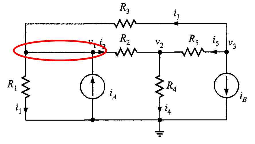
Se tiene el circuito mostrado en la figura 1. La dirección de las corrientes se asume tal como se ilustra en la figura.

Aplicando la LKC en el nodo 1, se tiene


Al usar la LKC en el nodo 2, resulta


Al usar la LKC en el nodo 3, resulta


Así que, las ecuaciones obtenidas son
 |
 |
 |
Recordando que 
 |
 |
 |
Se observa que el análisis produce tres ecuaciones simultáneas en las incógnitas 


La forma general general de la ecuación matricial es

La solución de la ecuación matricial es
donde la matriz inversa de 

El determinante de la matriz


La matriz adjunta de
![\displaystyle Adj \ \bold{G} = \left[\begin{matrix} C_{11} & C_{12} & C_{13} \\ C_{21} & C_{22} & C_{23} \\ C_{31} & C_{32} & C_{33} \end{matrix} \right]](https://s0.wp.com/latex.php?latex=%5Cdisplaystyle+Adj+%5C+%5Cbold%7BG%7D+%3D+%5Cleft%5B%5Cbegin%7Bmatrix%7D+C_%7B11%7D+%26+C_%7B12%7D+%26+C_%7B13%7D+%5C%5C+C_%7B21%7D+%26+C_%7B22%7D+%26+C_%7B23%7D+%5C%5C+C_%7B31%7D+%26+C_%7B32%7D+%26+C_%7B33%7D+%5Cend%7Bmatrix%7D+%5Cright%5D&bg=ffffff&fg=192930&s=0&c=20201002)
donde 

donde 

 |  |  |
 |  |  |
 |  |  |
Teniendo los resultados de cada menor, se puede calcular cada cofactor
 |  |  |
 |  |  |
 |  |  |
Nota. El determinante de cada menor no fue desarrollado ya que genera varios términos; sólo se expresará cuando se resuelva un problema donde implique matrices de 3×3.
Así, ya es posible conocer el resultado de la matriz adjunta de
![\displaystyle Adj \ \bold{G} = \left[\begin{matrix} C_{11} & C_{12} & C_{13} \\ C_{21} & C_{22} & C_{23} \\ C_{31} & C_{32} & C_{33} \end{matrix} \right] = \left[\begin{matrix} M_{11} & - M_{12} & M_{13} \\ - M_{21} & M_{22} &- M_{23} \\ M_{31} & - M_{32} & M_{33} \end{matrix} \right]](https://s0.wp.com/latex.php?latex=%5Cdisplaystyle+Adj+%5C+%5Cbold%7BG%7D+%3D+%5Cleft%5B%5Cbegin%7Bmatrix%7D+C_%7B11%7D+%26+C_%7B12%7D+%26+C_%7B13%7D+%5C%5C+C_%7B21%7D+%26+C_%7B22%7D+%26+C_%7B23%7D+%5C%5C+C_%7B31%7D+%26+C_%7B32%7D+%26+C_%7B33%7D+%5Cend%7Bmatrix%7D+%5Cright%5D+%3D+%5Cleft%5B%5Cbegin%7Bmatrix%7D+M_%7B11%7D+%26+-+M_%7B12%7D+%26+M_%7B13%7D+%5C%5C+-+M_%7B21%7D+%26+M_%7B22%7D+%26-++M_%7B23%7D+%5C%5C+M_%7B31%7D+%26+-+M_%7B32%7D+%26+M_%7B33%7D+%5Cend%7Bmatrix%7D+%5Cright%5D&bg=ffffff&fg=192930&s=0&c=20201002)
Una vez calculada la matriz adjunta, puede determinarse su traspuesta.
![\displaystyle {(Adj \ \bold{G})}^T = \left[\begin{matrix} M_{11} & - M_{21} & M_{31} \\ - M_{12} & M_{22} &- M_{32} \\ M_{13} & - M_{23} & M_{33} \end{matrix} \right]](https://s0.wp.com/latex.php?latex=%5Cdisplaystyle+%7B%28Adj+%5C+%5Cbold%7BG%7D%29%7D%5ET+%3D+%5Cleft%5B%5Cbegin%7Bmatrix%7D+M_%7B11%7D+%26+-+M_%7B21%7D+%26+M_%7B31%7D+%5C%5C+-+M_%7B12%7D+%26+M_%7B22%7D+%26-+M_%7B32%7D+%5C%5C+M_%7B13%7D+%26+-+M_%7B23%7D+%26+M_%7B33%7D+%5Cend%7Bmatrix%7D+%5Cright%5D&bg=ffffff&fg=192930&s=0&c=20201002)
Una vez calculado el determinante y la matriz adjunta traspuesta de
![\displaystyle \left[\begin{matrix} v_1 \\ v_2 \\ v_3 \end{matrix} \right] = \frac{{(Adj \ \bold{G})}^T}{\text{det} \ \bold{G}} \left[\begin{matrix} i_1 \\ i_2 \\ i_3 \end{matrix} \right] = \left(\frac{1}{\text{det} \ \bold{G}} \right) {(Adj \ \bold{G})}^T \left[\begin{matrix} i_1 \\ i_2 \\ i_3 \end{matrix} \right]](https://s0.wp.com/latex.php?latex=%5Cdisplaystyle+%5Cleft%5B%5Cbegin%7Bmatrix%7D+v_1+%5C%5C+v_2+%5C%5C+v_3+%5Cend%7Bmatrix%7D+%5Cright%5D+%3D+%5Cfrac%7B%7B%28Adj+%5C+%5Cbold%7BG%7D%29%7D%5ET%7D%7B%5Ctext%7Bdet%7D+%5C+%5Cbold%7BG%7D%7D+%5Cleft%5B%5Cbegin%7Bmatrix%7D+i_1+%5C%5C+i_2+%5C%5C+i_3+%5Cend%7Bmatrix%7D+%5Cright%5D+%3D+%5Cleft%28%5Cfrac%7B1%7D%7B%5Ctext%7Bdet%7D+%5C+%5Cbold%7BG%7D%7D+%5Cright%29+%7B%28Adj+%5C+%5Cbold%7BG%7D%29%7D%5ET+%5Cleft%5B%5Cbegin%7Bmatrix%7D+i_1+%5C%5C+i_2+%5C%5C+i_3+%5Cend%7Bmatrix%7D+%5Cright%5D+&bg=ffffff&fg=192930&s=0&c=20201002)
![\displaystyle \left[\begin{matrix} v_1 \\ v_2 \\ v_3 \end{matrix} \right] = \frac{1}{\left(g_{11} g_{22} g_{33} + g_{12} g_{23} g_{31} + g_{13} g_{21} g_{32} \right) - \left(g_{31} g_{22} g_{13} + g_{32} g_{23} g_{11} + g_{33} g_{21} g_{12} \right)} \left[\begin{matrix} M_{11} & - M_{21} & M_{31} \\ - M_{12} & M_{22} &- M_{32} \\ M_{13} & - M_{23} & M_{33} \end{matrix} \right] \left[\begin{matrix} i_1 \\ i_2 \\ i_3 \end{matrix} \right]](https://s0.wp.com/latex.php?latex=%5Cdisplaystyle+%5Cleft%5B%5Cbegin%7Bmatrix%7D+v_1+%5C%5C+v_2+%5C%5C+v_3+%5Cend%7Bmatrix%7D+%5Cright%5D+%3D+%5Cfrac%7B1%7D%7B%5Cleft%28g_%7B11%7D+g_%7B22%7D+g_%7B33%7D+%2B+g_%7B12%7D+g_%7B23%7D+g_%7B31%7D+%2B+g_%7B13%7D+g_%7B21%7D+g_%7B32%7D+%5Cright%29+-+%5Cleft%28g_%7B31%7D+g_%7B22%7D+g_%7B13%7D+%2B+g_%7B32%7D+g_%7B23%7D+g_%7B11%7D+%2B+g_%7B33%7D+g_%7B21%7D+g_%7B12%7D+%5Cright%29%7D+%5Cleft%5B%5Cbegin%7Bmatrix%7D+M_%7B11%7D+%26+-+M_%7B21%7D+%26+M_%7B31%7D+%5C%5C+-+M_%7B12%7D+%26+M_%7B22%7D+%26-+M_%7B32%7D+%5C%5C+M_%7B13%7D+%26+-+M_%7B23%7D+%26+M_%7B33%7D+%5Cend%7Bmatrix%7D+%5Cright%5D+%5Cleft%5B%5Cbegin%7Bmatrix%7D+i_1+%5C%5C+i_2+%5C%5C+i_3+%5Cend%7Bmatrix%7D+%5Cright%5D&bg=ffffff&fg=192930&s=0&c=20201002)
Problema resuelto
Problema 1. En la red de la figura 5, dados los valores siguientes, determine los voltajes de nodo: 


Aplicando la LKC en el nodo 1, se tiene


Usando la LKC para el nodo 2, se tiene que


Haciendo el mismo procedimiento para el nodo 3,


Entonces, el conjunto de ecuaciones son
 |
 |
 |
Recordando que
 |
 |
 |
Reduciendo
 |
 |
 |
Ahora, este sistema se puede expresar en forma matricial
![\displaystyle \left[ \begin{matrix} \frac{1}{1 \ \text{k}} & 0 & - \frac{1}{2 \ \text{k}} \\ \\ 0 & \frac{1}{2 \ \text{k}} & - \frac{1}{4 \ \text{k}} \\ \\ - \frac{1}{2 \ \text{k}} & - \frac{1}{4 \ \text{k}} & \frac{7}{4 \ \text{k}} \end{matrix} \right] \left[ \begin{matrix} v_1 \\ v_2 \\ v_3 \end{matrix} \right] = \left[ \begin{matrix} -4 \ \text{m} \\ 2 \ \text{m} \\ 0 \end{matrix} \right]](https://s0.wp.com/latex.php?latex=%5Cdisplaystyle+%5Cleft%5B+%5Cbegin%7Bmatrix%7D+%5Cfrac%7B1%7D%7B1+%5C+%5Ctext%7Bk%7D%7D+%26+0+%26+-+%5Cfrac%7B1%7D%7B2+%5C+%5Ctext%7Bk%7D%7D+%5C%5C+%5C%5C+0+%26+%5Cfrac%7B1%7D%7B2+%5C+%5Ctext%7Bk%7D%7D+%26+-+%5Cfrac%7B1%7D%7B4+%5C+%5Ctext%7Bk%7D%7D+%5C%5C+%5C%5C+-+%5Cfrac%7B1%7D%7B2+%5C+%5Ctext%7Bk%7D%7D+%26+-+%5Cfrac%7B1%7D%7B4+%5C+%5Ctext%7Bk%7D%7D+%26+%5Cfrac%7B7%7D%7B4+%5C+%5Ctext%7Bk%7D%7D+%5Cend%7Bmatrix%7D+%5Cright%5D+%5Cleft%5B+%5Cbegin%7Bmatrix%7D+v_1+%5C%5C+v_2+%5C%5C+v_3+%5Cend%7Bmatrix%7D+%5Cright%5D+%3D+%5Cleft%5B+%5Cbegin%7Bmatrix%7D+-4+%5C+%5Ctext%7Bm%7D+%5C%5C+2+%5C+%5Ctext%7Bm%7D+%5C%5C+0+%5Cend%7Bmatrix%7D+%5Cright%5D&bg=ffffff&fg=192930&s=0&c=20201002)
y esto es idéntico a
donde
![\displaystyle \bold{G} = \left[ \begin{matrix} \frac{1}{1 \ \text{k}} & 0 & - \frac{1}{2 \ \text{k}} \\ \\ 0 & \frac{1}{2 \ \text{k}} & - \frac{1}{4 \ \text{k}} \\ \\ - \frac{1}{2 \ \text{k}} & - \frac{1}{4 \ \text{k}} & \frac{7}{4 \ \text{k}} \end{matrix} \right]](https://s0.wp.com/latex.php?latex=%5Cdisplaystyle+%5Cbold%7BG%7D+%3D+%5Cleft%5B+%5Cbegin%7Bmatrix%7D+%5Cfrac%7B1%7D%7B1+%5C+%5Ctext%7Bk%7D%7D+%26+0+%26+-+%5Cfrac%7B1%7D%7B2+%5C+%5Ctext%7Bk%7D%7D+%5C%5C+%5C%5C+0+%26+%5Cfrac%7B1%7D%7B2+%5C+%5Ctext%7Bk%7D%7D+%26+-+%5Cfrac%7B1%7D%7B4+%5C+%5Ctext%7Bk%7D%7D+%5C%5C+%5C%5C+-+%5Cfrac%7B1%7D%7B2+%5C+%5Ctext%7Bk%7D%7D+%26+-+%5Cfrac%7B1%7D%7B4+%5C+%5Ctext%7Bk%7D%7D+%26+%5Cfrac%7B7%7D%7B4+%5C+%5Ctext%7Bk%7D%7D+%5Cend%7Bmatrix%7D+%5Cright%5D&bg=ffffff&fg=192930&s=0&c=20201002)
Para poder llegar a 


![\displaystyle \text{det} \ \bold{G} = \left[ \left(\frac{1}{1 \ \text{k}} \right) \left(\frac{1}{2 \ \text{k}} \right) \left(\frac{7}{4 \ \text{k}} \right) + \left(0 \right) \left(- \frac{1}{4 \ \text{k}}\right) \left(- \frac{1}{2 \ \text{k}} \right) + \left(-\frac{1}{2 \ \text{k}} \right) \left( 0 \right) \left(-\frac{1}{4 \ \text{k}} \right) \right] - \left[\left(-\frac{1}{2 \ \text{k}} \right) \left(\frac{1}{2 \ \text{k}} \right) \left(-\frac{1}{2 \ \text{k}} \right) + \left(-\frac{1}{4 \ \text{k}} \right) \left(-\frac{1}{4 \ \text{k}} \right) \left(\frac{1}{1 \ \text{k}} \right) + \left(\frac{7}{4 \ \text{k}} \right) \left(0 \right) \left(0 \right) \right]](https://s0.wp.com/latex.php?latex=%5Cdisplaystyle+%5Ctext%7Bdet%7D+%5C+%5Cbold%7BG%7D+%3D+%5Cleft%5B+%5Cleft%28%5Cfrac%7B1%7D%7B1+%5C+%5Ctext%7Bk%7D%7D+%5Cright%29+%5Cleft%28%5Cfrac%7B1%7D%7B2+%5C+%5Ctext%7Bk%7D%7D+%5Cright%29+%5Cleft%28%5Cfrac%7B7%7D%7B4+%5C+%5Ctext%7Bk%7D%7D+%5Cright%29+%2B+%5Cleft%280+%5Cright%29+%5Cleft%28-+%5Cfrac%7B1%7D%7B4+%5C+%5Ctext%7Bk%7D%7D%5Cright%29+%5Cleft%28-+%5Cfrac%7B1%7D%7B2+%5C+%5Ctext%7Bk%7D%7D+%5Cright%29+%2B+%5Cleft%28-%5Cfrac%7B1%7D%7B2+%5C+%5Ctext%7Bk%7D%7D+%5Cright%29+%5Cleft%28+0+%5Cright%29+%5Cleft%28-%5Cfrac%7B1%7D%7B4+%5C+%5Ctext%7Bk%7D%7D+%5Cright%29+%5Cright%5D+-+%5Cleft%5B%5Cleft%28-%5Cfrac%7B1%7D%7B2+%5C+%5Ctext%7Bk%7D%7D+%5Cright%29+%5Cleft%28%5Cfrac%7B1%7D%7B2+%5C+%5Ctext%7Bk%7D%7D+%5Cright%29+%5Cleft%28-%5Cfrac%7B1%7D%7B2+%5C+%5Ctext%7Bk%7D%7D+%5Cright%29+%2B+%5Cleft%28-%5Cfrac%7B1%7D%7B4+%5C+%5Ctext%7Bk%7D%7D+%5Cright%29+%5Cleft%28-%5Cfrac%7B1%7D%7B4+%5C+%5Ctext%7Bk%7D%7D+%5Cright%29+%5Cleft%28%5Cfrac%7B1%7D%7B1+%5C+%5Ctext%7Bk%7D%7D+%5Cright%29+%2B+%5Cleft%28%5Cfrac%7B7%7D%7B4+%5C+%5Ctext%7Bk%7D%7D+%5Cright%29+%5Cleft%280+%5Cright%29+%5Cleft%280+%5Cright%29+%5Cright%5D&bg=ffffff&fg=192930&s=0&c=20201002)


Para calcular la matriz adjunta de
es necesario calcular los menores (que pertenecen a cada cofactor).
 |  |  |
 |  |  |
 |  |  |
Entonces, los cofactores tiene los siguientes valores
 |  |  |
 |  |  |
 |  |  |
La matriz adjunta de
![\displaystyle Adj \ \bold{G} = \left[\begin{matrix} \frac{13}{16 \ \text{k}^2} & \frac{1}{8 \ \text{k}^2} & \frac{1}{4 \ \text{k}^2} \\ \\ \frac{1}{8 \ \text{k}^2} & \frac{3}{2 \ \text{k}^2} & \frac{1}{4 \ \text{k}^2} \\ \\ \frac{1}{4 \ \text{k}^2} & \frac{1}{4 \ \text{k}^2} & \frac{1}{2 \ \text{k}^2} \end{matrix} \right]](https://s0.wp.com/latex.php?latex=%5Cdisplaystyle+Adj+%5C+%5Cbold%7BG%7D+%3D+%5Cleft%5B%5Cbegin%7Bmatrix%7D+%5Cfrac%7B13%7D%7B16+%5C+%5Ctext%7Bk%7D%5E2%7D+%26+%5Cfrac%7B1%7D%7B8+%5C+%5Ctext%7Bk%7D%5E2%7D+%26+%5Cfrac%7B1%7D%7B4+%5C+%5Ctext%7Bk%7D%5E2%7D+%5C%5C+%5C%5C+%5Cfrac%7B1%7D%7B8+%5C+%5Ctext%7Bk%7D%5E2%7D+%26+%5Cfrac%7B3%7D%7B2+%5C+%5Ctext%7Bk%7D%5E2%7D+%26+%5Cfrac%7B1%7D%7B4+%5C+%5Ctext%7Bk%7D%5E2%7D+%5C%5C+%5C%5C+%5Cfrac%7B1%7D%7B4+%5C+%5Ctext%7Bk%7D%5E2%7D+%26+%5Cfrac%7B1%7D%7B4+%5C+%5Ctext%7Bk%7D%5E2%7D+%26+%5Cfrac%7B1%7D%7B2+%5C+%5Ctext%7Bk%7D%5E2%7D+%5Cend%7Bmatrix%7D+%5Cright%5D&bg=ffffff&fg=192930&s=0&c=20201002)
La matriz adjunta traspuesta de
![\displaystyle {(Adj \ \bold{G})}^T = \left[\begin{matrix} \frac{13}{16 \ \text{k}^2} & \frac{1}{8 \ \text{k}^2} & \frac{1}{4 \ \text{k}^2} \\ \\ \frac{1}{8 \ \text{k}^2} & \frac{3}{2 \ \text{k}^2} & \frac{1}{4 \ \text{k}^2} \\ \\ \frac{1}{4 \ \text{k}^2} & \frac{1}{4 \ \text{k}^2} & \frac{1}{2 \ \text{k}^2} \end{matrix} \right]](https://s0.wp.com/latex.php?latex=%5Cdisplaystyle+%7B%28Adj+%5C+%5Cbold%7BG%7D%29%7D%5ET+%3D+%5Cleft%5B%5Cbegin%7Bmatrix%7D+%5Cfrac%7B13%7D%7B16+%5C+%5Ctext%7Bk%7D%5E2%7D+%26+%5Cfrac%7B1%7D%7B8+%5C+%5Ctext%7Bk%7D%5E2%7D+%26+%5Cfrac%7B1%7D%7B4+%5C+%5Ctext%7Bk%7D%5E2%7D+%5C%5C+%5C%5C+%5Cfrac%7B1%7D%7B8+%5C+%5Ctext%7Bk%7D%5E2%7D+%26+%5Cfrac%7B3%7D%7B2+%5C+%5Ctext%7Bk%7D%5E2%7D+%26+%5Cfrac%7B1%7D%7B4+%5C+%5Ctext%7Bk%7D%5E2%7D+%5C%5C+%5C%5C+%5Cfrac%7B1%7D%7B4+%5C+%5Ctext%7Bk%7D%5E2%7D+%26+%5Cfrac%7B1%7D%7B4+%5C+%5Ctext%7Bk%7D%5E2%7D+%26+%5Cfrac%7B1%7D%7B2+%5C+%5Ctext%7Bk%7D%5E2%7D+%5Cend%7Bmatrix%7D+%5Cright%5D&bg=ffffff&fg=192930&s=0&c=20201002)
Calculando la matriz inversa

![\displaystyle \bold{G}^{-1} = \frac{1}{\frac{11}{16 \ \text{k}^3}} \left[\begin{matrix} \frac{13}{16 \ \text{k}^2} & \frac{1}{8 \ \text{k}^2} & \frac{1}{4 \ \text{k}^2} \\ \\ \frac{1}{8 \ \text{k}^2} & \frac{3}{2 \ \text{k}^2} & \frac{1}{4 \ \text{k}^2} \\ \\ \frac{1}{4 \ \text{k}^2} & \frac{1}{4 \ \text{k}^2} & \frac{1}{2 \ \text{k}^2} \end{matrix} \right] = \frac{16 \ \text{k}^3}{11} \left[\begin{matrix} \frac{13}{16 \ \text{k}^2} & \frac{1}{8 \ \text{k}^2} & \frac{1}{4 \ \text{k}^2} \\ \\ \frac{1}{8 \ \text{k}^2} & \frac{3}{2 \ \text{k}^2} & \frac{1}{4 \ \text{k}^2} \\ \\ \frac{1}{4 \ \text{k}^2} & \frac{1}{4 \ \text{k}^2} & \frac{1}{2 \ \text{k}^2} \end{matrix} \right]](https://s0.wp.com/latex.php?latex=%5Cdisplaystyle+%5Cbold%7BG%7D%5E%7B-1%7D+%3D+%5Cfrac%7B1%7D%7B%5Cfrac%7B11%7D%7B16+%5C+%5Ctext%7Bk%7D%5E3%7D%7D+%5Cleft%5B%5Cbegin%7Bmatrix%7D+%5Cfrac%7B13%7D%7B16+%5C+%5Ctext%7Bk%7D%5E2%7D+%26+%5Cfrac%7B1%7D%7B8+%5C+%5Ctext%7Bk%7D%5E2%7D+%26+%5Cfrac%7B1%7D%7B4+%5C+%5Ctext%7Bk%7D%5E2%7D+%5C%5C+%5C%5C+%5Cfrac%7B1%7D%7B8+%5C+%5Ctext%7Bk%7D%5E2%7D+%26+%5Cfrac%7B3%7D%7B2+%5C+%5Ctext%7Bk%7D%5E2%7D+%26+%5Cfrac%7B1%7D%7B4+%5C+%5Ctext%7Bk%7D%5E2%7D+%5C%5C+%5C%5C+%5Cfrac%7B1%7D%7B4+%5C+%5Ctext%7Bk%7D%5E2%7D+%26+%5Cfrac%7B1%7D%7B4+%5C+%5Ctext%7Bk%7D%5E2%7D+%26+%5Cfrac%7B1%7D%7B2+%5C+%5Ctext%7Bk%7D%5E2%7D+%5Cend%7Bmatrix%7D+%5Cright%5D+%3D+%5Cfrac%7B16+%5C+%5Ctext%7Bk%7D%5E3%7D%7B11%7D+%5Cleft%5B%5Cbegin%7Bmatrix%7D+%5Cfrac%7B13%7D%7B16+%5C+%5Ctext%7Bk%7D%5E2%7D+%26+%5Cfrac%7B1%7D%7B8+%5C+%5Ctext%7Bk%7D%5E2%7D+%26+%5Cfrac%7B1%7D%7B4+%5C+%5Ctext%7Bk%7D%5E2%7D+%5C%5C+%5C%5C+%5Cfrac%7B1%7D%7B8+%5C+%5Ctext%7Bk%7D%5E2%7D+%26+%5Cfrac%7B3%7D%7B2+%5C+%5Ctext%7Bk%7D%5E2%7D+%26+%5Cfrac%7B1%7D%7B4+%5C+%5Ctext%7Bk%7D%5E2%7D+%5C%5C+%5C%5C+%5Cfrac%7B1%7D%7B4+%5C+%5Ctext%7Bk%7D%5E2%7D+%26+%5Cfrac%7B1%7D%7B4+%5C+%5Ctext%7Bk%7D%5E2%7D+%26+%5Cfrac%7B1%7D%7B2+%5C+%5Ctext%7Bk%7D%5E2%7D+%5Cend%7Bmatrix%7D+%5Cright%5D&bg=ffffff&fg=192930&s=0&c=20201002)
![\displaystyle \bold{G}^{-1} = \left[\begin{matrix} \frac{16 \ \text{k}^3}{11} \left(\frac{13}{16 \ \text{k}^2} \right) & \frac{16 \ \text{k}^3}{11} \left(\frac{1}{8 \ \text{k}^2} \right) & \frac{16 \ \text{k}^3}{11} \left(\frac{1}{4 \ \text{k}^2} \right) \\ \\ \frac{16 \ \text{k}^3}{11} \left(\frac{1}{8 \ \text{k}^2} \right) & \frac{16 \ \text{k}^3}{11} \left(\frac{3}{2 \ \text{k}^2} \right) & \frac{16 \ \text{k}^3}{11} \left(\frac{1}{4 \ \text{k}^2} \right) \\ \\ \frac{16 \ \text{k}^3}{11} \left(\frac{1}{4 \ \text{k}^2} \right) & \frac{16 \ \text{k}^3}{11} \left(\frac{1}{4 \ \text{k}^2} \right) & \frac{16 \ \text{k}^3}{11} \left(\frac{1}{2 \ \text{k}^2} \right) \end{matrix} \right]](https://s0.wp.com/latex.php?latex=%5Cdisplaystyle+%5Cbold%7BG%7D%5E%7B-1%7D+%3D+%5Cleft%5B%5Cbegin%7Bmatrix%7D+%5Cfrac%7B16+%5C+%5Ctext%7Bk%7D%5E3%7D%7B11%7D+%5Cleft%28%5Cfrac%7B13%7D%7B16+%5C+%5Ctext%7Bk%7D%5E2%7D+%5Cright%29+%26+%5Cfrac%7B16+%5C+%5Ctext%7Bk%7D%5E3%7D%7B11%7D+%5Cleft%28%5Cfrac%7B1%7D%7B8+%5C+%5Ctext%7Bk%7D%5E2%7D+%5Cright%29+%26+%5Cfrac%7B16+%5C+%5Ctext%7Bk%7D%5E3%7D%7B11%7D+%5Cleft%28%5Cfrac%7B1%7D%7B4+%5C+%5Ctext%7Bk%7D%5E2%7D+%5Cright%29+%5C%5C+%5C%5C+%5Cfrac%7B16+%5C+%5Ctext%7Bk%7D%5E3%7D%7B11%7D+%5Cleft%28%5Cfrac%7B1%7D%7B8+%5C+%5Ctext%7Bk%7D%5E2%7D+%5Cright%29+%26+%5Cfrac%7B16+%5C+%5Ctext%7Bk%7D%5E3%7D%7B11%7D+%5Cleft%28%5Cfrac%7B3%7D%7B2+%5C+%5Ctext%7Bk%7D%5E2%7D+%5Cright%29+%26+%5Cfrac%7B16+%5C+%5Ctext%7Bk%7D%5E3%7D%7B11%7D+%5Cleft%28%5Cfrac%7B1%7D%7B4+%5C+%5Ctext%7Bk%7D%5E2%7D+%5Cright%29+%5C%5C+%5C%5C+%5Cfrac%7B16+%5C+%5Ctext%7Bk%7D%5E3%7D%7B11%7D+%5Cleft%28%5Cfrac%7B1%7D%7B4+%5C+%5Ctext%7Bk%7D%5E2%7D+%5Cright%29+%26+%5Cfrac%7B16+%5C+%5Ctext%7Bk%7D%5E3%7D%7B11%7D+%5Cleft%28%5Cfrac%7B1%7D%7B4+%5C+%5Ctext%7Bk%7D%5E2%7D+%5Cright%29+%26+%5Cfrac%7B16+%5C+%5Ctext%7Bk%7D%5E3%7D%7B11%7D+%5Cleft%28%5Cfrac%7B1%7D%7B2+%5C+%5Ctext%7Bk%7D%5E2%7D+%5Cright%29+%5Cend%7Bmatrix%7D+%5Cright%5D&bg=ffffff&fg=192930&s=0&c=20201002)
![\displaystyle \bold{G}^{-1} = \left[\begin{matrix} \frac{208}{176} \text{k} & \frac{16}{88} \text{k} & \frac{16}{44} \text{k} \\ \\ \frac{16}{88} \text{k} & \frac{48}{22} \text{k} & \frac{16}{44} \text{k} \\ \\ \frac{16}{44} \text{k} & \frac{16}{44} \text{k} & \frac{16}{22} \text{k} \end{matrix} \right] = \left[\begin{matrix} \frac{13}{11} \text{k} & \frac{2}{11} \text{k} & \frac{4}{11} \text{k} \\ \\ \frac{2}{11} \text{k} & \frac{24}{11} \text{k} & \frac{4}{11} \text{k} \\ \\ \frac{4}{11} \text{k} & \frac{4}{11} \text{k} & \frac{8}{11} \text{k} \end{matrix} \right]](https://s0.wp.com/latex.php?latex=%5Cdisplaystyle+%5Cbold%7BG%7D%5E%7B-1%7D+%3D+%5Cleft%5B%5Cbegin%7Bmatrix%7D+%5Cfrac%7B208%7D%7B176%7D+%5Ctext%7Bk%7D+%26+%5Cfrac%7B16%7D%7B88%7D+%5Ctext%7Bk%7D+%26+%5Cfrac%7B16%7D%7B44%7D+%5Ctext%7Bk%7D+%5C%5C+%5C%5C+%5Cfrac%7B16%7D%7B88%7D+%5Ctext%7Bk%7D+%26+%5Cfrac%7B48%7D%7B22%7D+%5Ctext%7Bk%7D+%26+%5Cfrac%7B16%7D%7B44%7D+%5Ctext%7Bk%7D+%5C%5C+%5C%5C+%5Cfrac%7B16%7D%7B44%7D+%5Ctext%7Bk%7D+%26+%5Cfrac%7B16%7D%7B44%7D+%5Ctext%7Bk%7D+%26+%5Cfrac%7B16%7D%7B22%7D+%5Ctext%7Bk%7D+%5Cend%7Bmatrix%7D+%5Cright%5D+%3D+%5Cleft%5B%5Cbegin%7Bmatrix%7D+%5Cfrac%7B13%7D%7B11%7D+%5Ctext%7Bk%7D+%26+%5Cfrac%7B2%7D%7B11%7D+%5Ctext%7Bk%7D+%26+%5Cfrac%7B4%7D%7B11%7D+%5Ctext%7Bk%7D+%5C%5C+%5C%5C+%5Cfrac%7B2%7D%7B11%7D+%5Ctext%7Bk%7D+%26+%5Cfrac%7B24%7D%7B11%7D+%5Ctext%7Bk%7D+%26+%5Cfrac%7B4%7D%7B11%7D+%5Ctext%7Bk%7D+%5C%5C+%5C%5C+%5Cfrac%7B4%7D%7B11%7D+%5Ctext%7Bk%7D+%26+%5Cfrac%7B4%7D%7B11%7D+%5Ctext%7Bk%7D+%26+%5Cfrac%7B8%7D%7B11%7D+%5Ctext%7Bk%7D+%5Cend%7Bmatrix%7D+%5Cright%5D&bg=ffffff&fg=192930&s=0&c=20201002)
Entonces, la forma matricial desarrollada es
![\displaystyle \left[\begin{matrix} v_1 \\ v_2 \\ v_3 \end{matrix} \right] = \left[\begin{matrix} \frac{13}{11} \text{k} & \frac{2}{11} \text{k} & \frac{4}{11} \text{k} \\ \\ \frac{2}{11} \text{k} & \frac{24}{11} \text{k} & \frac{4}{11} \text{k} \\ \\ \frac{4}{11} \text{k} & \frac{4}{11} \text{k} & \frac{8}{11} \text{k} \end{matrix} \right] \left[ \begin{matrix} -4 \ \text{m} \\ 2 \ \text{m} \\ 0 \end{matrix} \right]](https://s0.wp.com/latex.php?latex=%5Cdisplaystyle+%5Cleft%5B%5Cbegin%7Bmatrix%7D+v_1+%5C%5C+v_2+%5C%5C+v_3+%5Cend%7Bmatrix%7D+%5Cright%5D+%3D+%5Cleft%5B%5Cbegin%7Bmatrix%7D+%5Cfrac%7B13%7D%7B11%7D+%5Ctext%7Bk%7D+%26+%5Cfrac%7B2%7D%7B11%7D+%5Ctext%7Bk%7D+%26+%5Cfrac%7B4%7D%7B11%7D+%5Ctext%7Bk%7D+%5C%5C+%5C%5C+%5Cfrac%7B2%7D%7B11%7D+%5Ctext%7Bk%7D+%26+%5Cfrac%7B24%7D%7B11%7D+%5Ctext%7Bk%7D+%26+%5Cfrac%7B4%7D%7B11%7D+%5Ctext%7Bk%7D+%5C%5C+%5C%5C+%5Cfrac%7B4%7D%7B11%7D+%5Ctext%7Bk%7D+%26+%5Cfrac%7B4%7D%7B11%7D+%5Ctext%7Bk%7D+%26+%5Cfrac%7B8%7D%7B11%7D+%5Ctext%7Bk%7D+%5Cend%7Bmatrix%7D+%5Cright%5D+%5Cleft%5B+%5Cbegin%7Bmatrix%7D+-4+%5C+%5Ctext%7Bm%7D+%5C%5C+2+%5C+%5Ctext%7Bm%7D+%5C%5C+0+%5Cend%7Bmatrix%7D+%5Cright%5D&bg=ffffff&fg=192930&s=0&c=20201002)
Realizando la multiplicación matricial en el segundo miembro, resulta
![\displaystyle \left[\begin{matrix} v_1 \\ v_2 \\ v_3 \end{matrix} \right] = \left[\begin{matrix} \left(\frac{13}{11} \text{k} \right) (-4 \ \text{m}) + \left(\frac{2}{11} \text{k} \right) (2 \ \text{m}) + \left(\frac{4}{11} \text{k} \right) (0) \\ \\ \left(\frac{2}{11} \text{k} \right) (-4 \ \text{m}) + \left(\frac{24}{11} \text{k} \right) (2 \ \text{m}) + \left(\frac{4}{11} \text{k} \right) (0) \\ \\ \left(\frac{4}{11} \text{k} \right)(-4 \ \text{m}) + \left(\frac{4}{11} \text{k} \right)(2 \ \text{m}) + \left(\frac{8}{11} \text{k} \right) (0) \end{matrix} \right]](https://s0.wp.com/latex.php?latex=%5Cdisplaystyle+%5Cleft%5B%5Cbegin%7Bmatrix%7D+v_1+%5C%5C+v_2+%5C%5C+v_3+%5Cend%7Bmatrix%7D+%5Cright%5D+%3D+%5Cleft%5B%5Cbegin%7Bmatrix%7D+%5Cleft%28%5Cfrac%7B13%7D%7B11%7D+%5Ctext%7Bk%7D+%5Cright%29+%28-4+%5C+%5Ctext%7Bm%7D%29+%2B+%5Cleft%28%5Cfrac%7B2%7D%7B11%7D+%5Ctext%7Bk%7D+%5Cright%29+%282+%5C+%5Ctext%7Bm%7D%29+%2B+%5Cleft%28%5Cfrac%7B4%7D%7B11%7D+%5Ctext%7Bk%7D+%5Cright%29+%280%29+%5C%5C+%5C%5C+%5Cleft%28%5Cfrac%7B2%7D%7B11%7D+%5Ctext%7Bk%7D+%5Cright%29+%28-4+%5C+%5Ctext%7Bm%7D%29+%2B+%5Cleft%28%5Cfrac%7B24%7D%7B11%7D+%5Ctext%7Bk%7D+%5Cright%29+%282+%5C+%5Ctext%7Bm%7D%29+%2B+%5Cleft%28%5Cfrac%7B4%7D%7B11%7D+%5Ctext%7Bk%7D+%5Cright%29+%280%29+%5C%5C+%5C%5C+%5Cleft%28%5Cfrac%7B4%7D%7B11%7D+%5Ctext%7Bk%7D+%5Cright%29%28-4+%5C+%5Ctext%7Bm%7D%29+%2B+%5Cleft%28%5Cfrac%7B4%7D%7B11%7D+%5Ctext%7Bk%7D+%5Cright%29%282+%5C+%5Ctext%7Bm%7D%29+%2B+%5Cleft%28%5Cfrac%7B8%7D%7B11%7D+%5Ctext%7Bk%7D+%5Cright%29+%280%29+%5Cend%7Bmatrix%7D+%5Cright%5D&bg=ffffff&fg=192930&s=0&c=20201002)
recordando que 

![\displaystyle \left[\begin{matrix} v_1 \\ v_2 \\ v_3 \end{matrix} \right] = \left[\begin{matrix} \left(\frac{13}{11} \times 10^3 \right) (-4 \times 10^{-3}) + \left(\frac{2}{11} \times 10^{3} \right) (2 \times 10^{-3}) + \left(\frac{4}{11} \times 10^{3} \right) (0) \\ \\ \left(\frac{2}{11} \times 10^{3} \right) (-4 \times 10^{-3}) + \left(\frac{24}{11} \times 10^{3} \right) (2 \times 10^{-3}) + \left(\frac{4}{11} \times 10^{3} \right) (0) \\ \\ \left(\frac{4}{11} \times 10^{3} \right)(-4 \times 10^{-3}) + \left(\frac{4}{11} \times 10^{3} \right)(2 \times 10^{-3}) + \left(\frac{8}{11} \times 10^{3} \right) (0) \end{matrix} \right]](https://s0.wp.com/latex.php?latex=%5Cdisplaystyle+%5Cleft%5B%5Cbegin%7Bmatrix%7D+v_1+%5C%5C+v_2+%5C%5C+v_3+%5Cend%7Bmatrix%7D+%5Cright%5D+%3D+%5Cleft%5B%5Cbegin%7Bmatrix%7D+%5Cleft%28%5Cfrac%7B13%7D%7B11%7D+%5Ctimes+10%5E3+%5Cright%29+%28-4+%5Ctimes+10%5E%7B-3%7D%29+%2B+%5Cleft%28%5Cfrac%7B2%7D%7B11%7D+%5Ctimes+10%5E%7B3%7D+%5Cright%29+%282+%5Ctimes+10%5E%7B-3%7D%29+%2B+%5Cleft%28%5Cfrac%7B4%7D%7B11%7D+%5Ctimes+10%5E%7B3%7D+%5Cright%29+%280%29+%5C%5C+%5C%5C+%5Cleft%28%5Cfrac%7B2%7D%7B11%7D+%5Ctimes+10%5E%7B3%7D+%5Cright%29+%28-4+%5Ctimes+10%5E%7B-3%7D%29+%2B+%5Cleft%28%5Cfrac%7B24%7D%7B11%7D+%5Ctimes+10%5E%7B3%7D+%5Cright%29+%282+%5Ctimes+10%5E%7B-3%7D%29+%2B+%5Cleft%28%5Cfrac%7B4%7D%7B11%7D+%5Ctimes+10%5E%7B3%7D+%5Cright%29+%280%29+%5C%5C+%5C%5C+%5Cleft%28%5Cfrac%7B4%7D%7B11%7D+%5Ctimes+10%5E%7B3%7D+%5Cright%29%28-4+%5Ctimes+10%5E%7B-3%7D%29+%2B+%5Cleft%28%5Cfrac%7B4%7D%7B11%7D+%5Ctimes+10%5E%7B3%7D+%5Cright%29%282+%5Ctimes+10%5E%7B-3%7D%29+%2B+%5Cleft%28%5Cfrac%7B8%7D%7B11%7D+%5Ctimes+10%5E%7B3%7D+%5Cright%29+%280%29+%5Cend%7Bmatrix%7D+%5Cright%5D&bg=ffffff&fg=192930&s=0&c=20201002)
![\displaystyle \left[\begin{matrix} v_1 \\ v_2 \\ v_3 \end{matrix} \right] = \left[\begin{matrix} -\frac{52}{11} + \frac{4}{11} + 0 \\ \\ -\frac{8}{11} + \frac{48}{11} + 0 \\ \\ - \frac{16}{11} + \frac{8}{11} + 0 \end{matrix} \right] = \left[\begin{matrix} - \frac{48}{11} \\ \\ \frac{40}{11} \\ \\ - \frac{8}{11} \end{matrix} \right]](https://s0.wp.com/latex.php?latex=%5Cdisplaystyle+%5Cleft%5B%5Cbegin%7Bmatrix%7D+v_1+%5C%5C+v_2+%5C%5C+v_3+%5Cend%7Bmatrix%7D+%5Cright%5D+%3D+%5Cleft%5B%5Cbegin%7Bmatrix%7D+-%5Cfrac%7B52%7D%7B11%7D+%2B+%5Cfrac%7B4%7D%7B11%7D+%2B+0+%5C%5C+%5C%5C+-%5Cfrac%7B8%7D%7B11%7D+%2B+%5Cfrac%7B48%7D%7B11%7D+%2B+0+%5C%5C+%5C%5C+-+%5Cfrac%7B16%7D%7B11%7D+%2B+%5Cfrac%7B8%7D%7B11%7D+%2B+0+%5Cend%7Bmatrix%7D+%5Cright%5D+%3D+%5Cleft%5B%5Cbegin%7Bmatrix%7D+-+%5Cfrac%7B48%7D%7B11%7D+%5C%5C+%5C%5C++%5Cfrac%7B40%7D%7B11%7D+%5C%5C+%5C%5C+-+%5Cfrac%7B8%7D%7B11%7D+%5Cend%7Bmatrix%7D+%5Cright%5D&bg=ffffff&fg=192930&s=0&c=20201002)
![\displaystyle \therefore \left[\begin{matrix} v_1 \\ v_2 \\ v_3 \end{matrix} \right] = \left[\begin{matrix} -4.3636 \\ \\ 3.6364 \\ \\ - 0.7273 \end{matrix} \right] \ \text{V}](https://s0.wp.com/latex.php?latex=%5Cdisplaystyle+%5Ctherefore+%5Cleft%5B%5Cbegin%7Bmatrix%7D+v_1+%5C%5C+v_2+%5C%5C+v_3+%5Cend%7Bmatrix%7D+%5Cright%5D+%3D+%5Cleft%5B%5Cbegin%7Bmatrix%7D+-4.3636+%5C%5C+%5C%5C+3.6364+%5C%5C+%5C%5C+-+0.7273+%5Cend%7Bmatrix%7D+%5Cright%5D+%5C+%5Ctext%7BV%7D&bg=ffffff&fg=192930&s=0&c=20201002)
Se concluye que los voltajes de cada nodo son 


