Teorema de Thévenin y de Norton para circuitos que incluyen únicamente fuentes independientes. Circuitos eléctricos.

Problemas resueltos

Problema 1. Encontrar $V_o$ en la red de la figura 1.

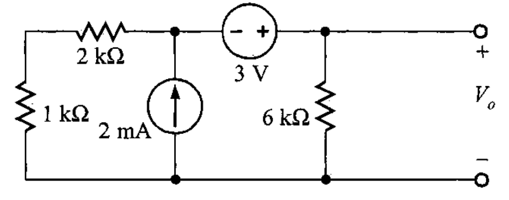
Primer método. Utilizando el teorema de Thévenin.

Solución. Para determinar el circuito equivalente de Thévenin se abre la red en la carga de 6 kΩ (figura 2).

La LKV indica que el voltaje en circuito abierto, $V_{oc}$ , es igual a 3 V más el voltaje $V_1$ , que es el voltaje en las terminales de la fuente de corriente. Los 2 mA de la fuente de corriente fluyen a través de los resistores, por lo que el valor de $V_1$ es

$\displaystyle V_1 = (2 \ \text{k} + 1 \ \text{k}) (2 \ \text{m})$

$\displaystyle V_1 = (3 \ \text{k}) (2 \ \text{m}) = (3 \times 10^3) (2 \times 10^{-3})$

$\displaystyle V_1 = 6 \ \text{V}$

Entonces, $V_{oc}$ es

$\displaystyle V_{oc} = 3 \ \text{V} + V_1 = 3 + 6 = 9 \ \text{V}$

$\displaystyle V_{oc} = 9 \ \text{V}$

Después, todas las fuentes de corriente del circuito se cambian a circuitos abiertos mientras que las fuentes de voltaje se cambian a cortocircuitos; con esto se puede hallar la resistencia equivalente de Thévenin (figura 3).

$\displaystyle R_{\text{Th}} = 2 \ \text{k} + 1 \ \text{k}$

$\displaystyle R_{\text{Th}} = 3 \ \text{k} \Omega$

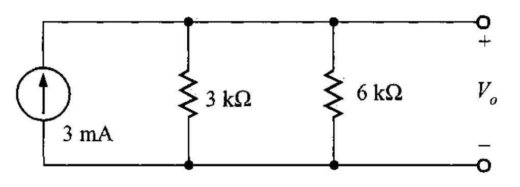
Luego, se conecta el circuito equivalente de Thévenin formado por $V_{oc}$ y $R_{\text{Th}}$ en las terminales originales de la carga (figura 4).

Figura 4. Conexión del circuito equivalente de Thévenin con la carga y el voltaje Vo.

Por último, por divisor de voltaje, se calcula el valor de $V_o$ .

$\displaystyle V_o = \left(\frac{6 \ \text{k}}{3 \ \text{k} + 6 \ \text{k}} \right) (9)$

$\displaystyle V_o = \left(\frac{6 \ \text{k}}{9 \ \text{k}} \right) (9) = 6$

$\displaystyle \therefore V_o = 6 \ \text{V}$

Segundo método. Utilizando el teorema de Norton.

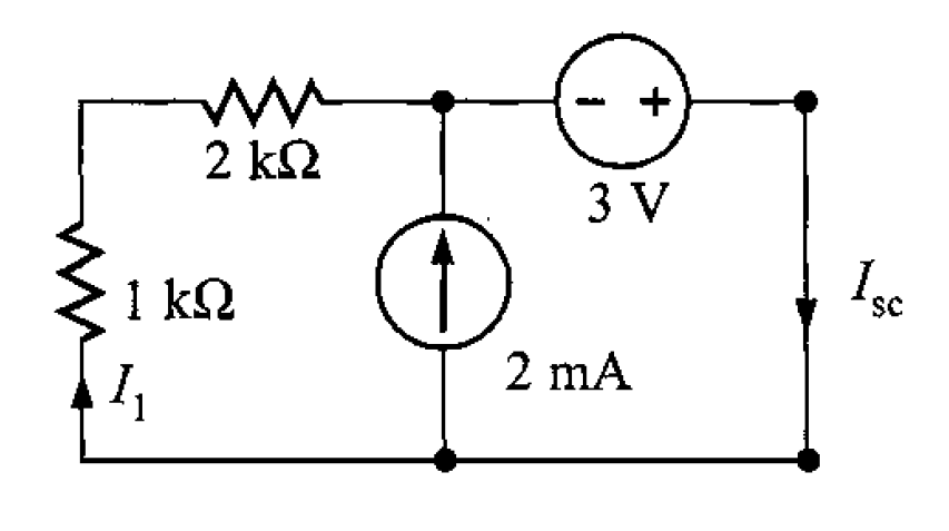
Solución. Para el circuito equivalente de Norton en las terminales de la carga, se debe calcular la corriente de cortocircuito, como se muestra en la figura 5. Se observa que el cortocircuito hace que la fuente de 3 V quede directamente entre los resistores y la fuente de corriente (esto es, en paralelo con dichos elementos).

Entonces, $I_1$ es

$\displaystyle I_1 = \frac{3}{2 \ \text{k} + 1 \ \text{k}}$

$\displaystyle I_1 = \frac{3}{3 \ \text{k}} = \frac{3}{3 \times 10^{3}} = 1 \times 10^{-3}$

$\displaystyle I_1 = 1 \ \text{mA}$

Aplicando la LKC en la figura 5, resulta

$\displaystyle \sum_{j=1}^n{I_j} = 0$

$\displaystyle -I_1 - 2 \ \text{m} + I_{sc} = 0$

$\displaystyle I_{sc} = I_1 + 2 \ \text{m} = 1 \ \text{m} + 2 \ \text{m}$

$\displaystyle I_{sc} = 3 \ \text{mA}$

El valor de $R_{\text{Th}}$ se determinó en el desarrollo del teorema de Thévenin en base a la figura 3; esto es $R_{\text{Th}} = 3 \ \text{k} \Omega$ . Finalmente, conectando el circuito equivalente de Norton formado por $I_{sc}$ y $R_{\text{Th}}$ se tiene el circuito mostrado en la figura 6.

Figura 6. Conexión del circuito equivalente de Norton con la carga y el voltaje V_o.

Por ley de Ohm, se obtiene el valor de $V_o$ . Esto es

$\displaystyle V_o = \left[\frac{(3 \ \text{k})(6 \ \text{k})}{3 \ \text{k} + 6 \ \text{k}} \right] (3 \ \text{m})$

$\displaystyle V_o = \left(\frac{18}{9} \ \text{k} \right) (3 \ \text{m}) = \left(2 \ \text{k} \right) (3 \ \text{m}) = \left(2 \times 10^3 \right) (3 \times 10^{-3})$

$\displaystyle \therefore V_o = 6 \ \text{V}$

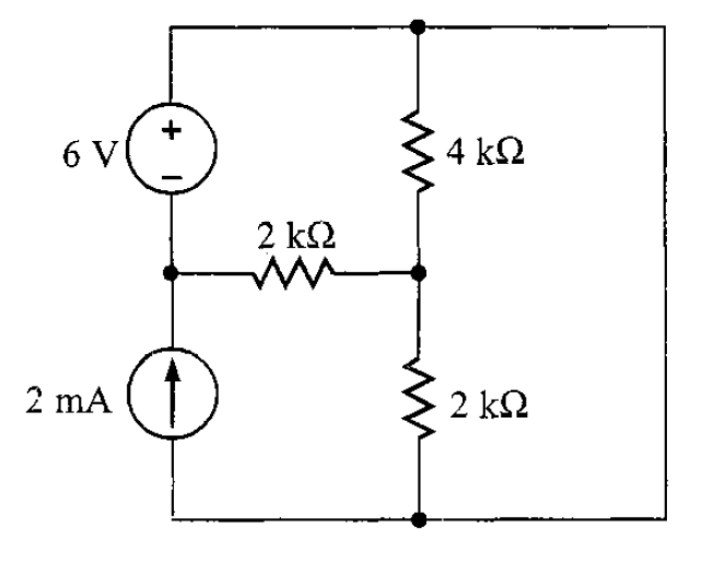
Problema 2. Hallar el valor de $V_o$ para el circuito de la figura 7.

Primer método. Utilizando el teorema de Thévenin.

Solución. Se abre la red en la carga de 6 kΩ; esto genera dos mallas, como se observa en la figura 8.

La ecuación para la primera corriente de malla es

$\displaystyle \sum_{j = 1}^n{V_j} = 0$

$\displaystyle -6 + (4 \ \text{k})I_1 + (2 \ \text{k}) (I_1 - I_2) = 0$

$\displaystyle - 6 + (4 \ \text{k})I_1 + (2 \ \text{k}) I_1 - (2 \ \text{k}) I_2 = 0$

$\displaystyle (6 \ \text{k})I_1 - (2 \ \text{k}) I_2 = 6$

Y la segunda corriente de malla es

$\displaystyle I_2 = 2 \ \text{mA} = 2 \times 10^{-3} \ \text{A}$

Teniendo las ecuaciones

\displaystyle (6 \ \text{k})I_1 - (2 \ \text{k}) I_2 = 6

Sustituyendo la ecuación (2) en (1), resulta que

$\displaystyle (6 \ \text{k})I_1 - (2 \ \text{k}) I_2 = 6$

$\displaystyle (6 \ \text{k})I_1 - (2 \ \text{k}) (2 \times 10^{-3}) = 6$

$\displaystyle (6 \times 10^3)I_1 - 4 = 6$

$\displaystyle (6 \times 10^3)I_1 = 10$

$\displaystyle I_1 = \frac{10}{6 \times 10^3} = \frac{5}{3} \times 10^{-3}$

$\displaystyle I_1 = \frac{5}{3} \ \text{mA}$

Una vez calculado los valores de las corrientes $I_1$ e $I_2$ , se utiliza LKV para determinar $V_{oc}$ .

$\displaystyle \sum_{j=1}^n{V_j} = 0$

$\displaystyle - (2 \ \text{k})I_2 - (4 \ \text{k}) I_1 + V_{oc} = 0$

$\displaystyle V_{oc} = (4 \ \text{k}) I_1 + (2 \ \text{k})I_2$

$\displaystyle V_{oc} = (4 \times 10^3) \left(\frac{5}{3} \times 10^{-3} \right) + (2 \times 10^3) (2 \times 10^{-3}) = \frac{20}{3} + 4 = \frac{32}{3}$

$\displaystyle V_{oc} = \frac{32}{3} \ \text{V}$

Haciendo que la fuente de voltaje se comporte como un cortocircuito y que la fuente de corriente como un circuito abierto, se tiene lo siguiente en la figura 9.

Figura 9. Determinando la resistencia de Thévenin R_Th.

Con esto es posible determinar la resistencia Thévenin y es

$\displaystyle R_{\text{Th}} = \frac{(2 \ \text{k})(4 \ \text{k})}{2 \ \text{k} + 4 \ \text{k}} + 2 \ \text{k}$

$\displaystyle R_{\text{Th}} = \frac{8}{6} \ \text{k} + 2 \ \text{k} = \frac{4}{3} \ \text{k} + 2 \ \text{k}$

$\displaystyle R_{\text{Th}} = \frac{10}{3} \ \text{k} \Omega$

Conectando el circuito equivalente de Thévenin a la carga se produce el circuito mostrado en la figura 10.

Figura 10. Conexión del circuito equivalente de Thévenin a la carga.

Usando la división de voltaje, se obtiene el resultado final de $V_o$ .

$\displaystyle V_o = \left(\frac{6 \ \text{k}}{\frac{10}{3} \ \text{k} + 6 \ \text{k}} \right) \left(\frac{32}{3} \right)$

$\displaystyle V_o = \left(\frac{6 \ \text{k}}{\frac{28}{3} \ \text{k}} \right) \left(\frac{32}{3} \right)$

$\displaystyle V_o = \left(\frac{18}{28} \right) \left(\frac{32}{3} \right) = \frac{48}{7}$

$\displaystyle \therefore V_o = \frac{48}{7} \ \text{V}$

Segundo método. Utilizando el teorema de Norton.

Solución. Para ello, es necesario que en las terminales de la carga, se determine la corriente de cortocircuito, como se ilustra en la figura 11.

Figura 11. Procedimiento para hallar el circuito equivalente de Norton.

Figura 12. Asignando las corrientes de malla del circuito de la figura 11.

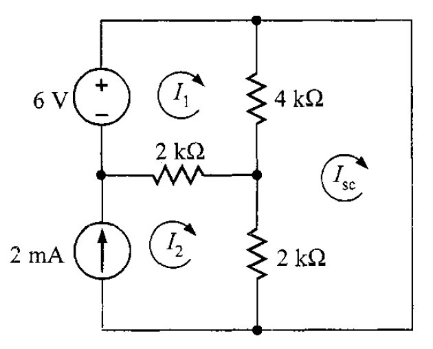
En la figura 12 se observa que se han localizado las corrientes de malla y pueden ser hallas utilizando la LKV. En la primera corriente de malla, su ecuación es

$\displaystyle \sum_{j=1}^n{V_j} = 0$

$\displaystyle - 6 + (4 \ \text{k}) (I_1 - I_{sc}) + (2 \ \text{k})(I_1 - I_2) = 0$

$\displaystyle - 6 + (4 \ \text{k}) I_1 - (4 \ \text{k}) I_{sc} + (2 \ \text{k}) I_1 - (2 \ \text{k}) I_2 = 0$

$\displaystyle (6 \ \text{k}) I_1 - (2 \ \text{k}) I_2 - (4 \ \text{k}) I_{sc} = 6$

La ecuación de la segunda corriente de malla es

$\displaystyle I_2 = 2 \ \text{mA} = 2 \times 10^{-3} \ \text{A}$

y en le caso de la tercera corriente de malla

$\displaystyle \sum_{j=1}^n{V_j} = 0$

$\displaystyle (2 \ \text{k})(I_{sc} - I_2) + (4 \ \text{k})(I_{sc} - I_1) = 0$

$\displaystyle (2 \ \text{k}) I_{sc} - (2 \ \text{k}) I_2 + (4 \ \text{k}) I_{sc} - (4 \ \text{k}) I_1 = 0$

$\displaystyle - (4 \ \text{k}) I_1 - (2 \ \text{k}) I_2 + (6 \ \text{k}) I_{sc} = 0$

Las ecuaciones obtenidas anteriormente son

\displaystyle (6 \ \text{k}) I_1 - (2 \ \text{k}) I_2 - (4 \ \text{k}) I_{sc} = 6

Sustituyendo de la ecuación (2) en (1) y (3), se reduce a dos ecuaciones

\displaystyle (6 \ \text{k}) I_1 - (2 \ \text{k}) (2 \times 10^{-3}) - (4 \ \text{k}) I_{sc} = 6

\displaystyle - (4 \ \text{k}) I_1 - (2 \ \text{k}) (2 \times 10^{-3}) + (6 \ \text{k}) I_{sc} = 0

Simplificando

\displaystyle (6 \ \text{k}) I_1 - (4 \ \text{k}) I_{sc} = 10

\displaystyle - (4 \ \text{k}) I_1 + (6 \ \text{k}) I_{sc} = 4

Con esto sólo es necesario determinar $I_1$ e $I_{sc}$ . Expresando las ecuaciones (4) y (5) en forma matricial, se tiene lo siguiente

$\displaystyle \left[\begin{matrix} 6 \ \text{k} & -4\ \text{k} \\ -4 \ \text{k} & 6 \ \text{k} \end{matrix} \right] \left[\begin{matrix} I_1 \\ I_{sc} \end{matrix} \right] = \left[\begin{matrix} 10 \\ 4 \end{matrix} \right]$

$\displaystyle \left[\begin{matrix} I_1 \\ I_{sc} \end{matrix} \right] = {\left[\begin{matrix} 6 \ \text{k} & -4\ \text{k} \\ -4 \ \text{k} & 6 \ \text{k} \end{matrix} \right]}^{-1} \left[\begin{matrix} 10 \\ 4 \end{matrix} \right]$

$\displaystyle \left[\begin{matrix} I_1 \\ I_{sc} \end{matrix} \right] = \left(\frac{1}{20 \ \text{k}^2} \right) \left[\begin{matrix} 6 \ \text{k} & 4\ \text{k} \\ 4 \ \text{k} & 6 \ \text{k} \end{matrix} \right] \left[\begin{matrix} 10 \\ 4 \end{matrix} \right]$

$\displaystyle \left[\begin{matrix} I_1 \\ I_{sc} \end{matrix} \right] = \left[\begin{matrix} \left(\frac{1}{20 \ \text{k}^2} \right)(6 \ \text{k}) & \left(\frac{1}{20 \ \text{k}^2} \right)(4\ \text{k}) \\ \left(\frac{1}{20 \ \text{k}^2} \right)(4 \ \text{k}) & \left(\frac{1}{20 \ \text{k}^2} \right)(6 \ \text{k}) \end{matrix} \right] \left[\begin{matrix} 10 \\ 4 \end{matrix} \right]$

$\displaystyle \left[\begin{matrix} I_1 \\ I_{sc} \end{matrix} \right] = \left[\begin{matrix} \frac{6}{20 \ \text{k}} & \frac{4}{20 \ \text{k}} \\ \frac{4}{20 \ \text{k}} &\frac{6}{20 \ \text{k}} \end{matrix} \right] \left[\begin{matrix} 10 \\ 4 \end{matrix} \right] = \left[\begin{matrix} \frac{6}{20 \times 10^{3}} & \frac{4}{20 \times 10^{3}} \\ \frac{4}{20 \times 10^{3}} &\frac{6}{20 \times 10^{3}} \end{matrix} \right] \left[\begin{matrix} 10 \\ 4 \end{matrix} \right]$

$\displaystyle \left[\begin{matrix} I_1 \\ I_{sc} \end{matrix} \right] = \left[\begin{matrix} \frac{3}{10} \times 10^{-3} & \frac{1}{5} \times 10^{-3} \\ \\ \frac{1}{5} \times 10^{-3} &\frac{3}{10} \times 10^{-3} \end{matrix} \right] \left[\begin{matrix} 10 \\ 4 \end{matrix} \right] = \left[\begin{matrix} \left(\frac{3}{10} \times 10^{-3} \right)(10) + \left(\frac{1}{5} \times 10^{-3} \right)(4) \\ \\ \left(\frac{1}{5} \times 10^{-3} \right)(10) + \left(\frac{3}{10} \times 10^{-3}\right)(4) \end{matrix} \right]$

$\displaystyle \left[\begin{matrix} I_1 \\ I_{sc} \end{matrix} \right] = \left[\begin{matrix} 3 \times 10^{-3} + \frac{4}{5} \times 10^{-3} \\ \\ 2 \times 10^{-3} + \frac{6}{5} \times 10^{-3} \end{matrix} \right] = \left[\begin{matrix} \frac{19}{5} \times 10^{-3} \\ \\ \frac{16}{5} \times 10^{-3} \end{matrix} \right] = \left[\begin{matrix} \frac{19}{5} \\ \\ \frac{16}{5} \end{matrix} \right] \times 10^{-3}$

$\displaystyle \left[\begin{matrix} I_1 \\ I_{sc} \end{matrix} \right] = \left[\begin{matrix} \frac{19}{5} \\ \\ \frac{16}{5} \end{matrix} \right] \ \text{mA}$

Entonces las corrientes son $\displaystyle I_1 =\frac{19}{5} \ \text{mA}$ y $\displaystyle I_{sc} =\frac{16}{5} \ \text{mA}$ .

La resistencia Thévenin se determinó cuando las fuentes de voltaje y corriente se volvieron nulas cuando se estaba encontrando el circuito equivalente de Thévenin. Entonces, $R_{\text{Th}}$ es

$\displaystyle R_{\text{Th}} = \frac{(2 \ \text{k})(4 \ \text{k})}{2 \ \text{k} + 4 \ \text{k}} + 2 \ \text{k}$

$\displaystyle R_{\text{Th}} = \frac{10}{3} \ \text{k} \Omega$

Por último, se conecta el circuito equivalente de Norton a la carga que fue separada en un principio; el circuito esperado se muestra en la figura 13.

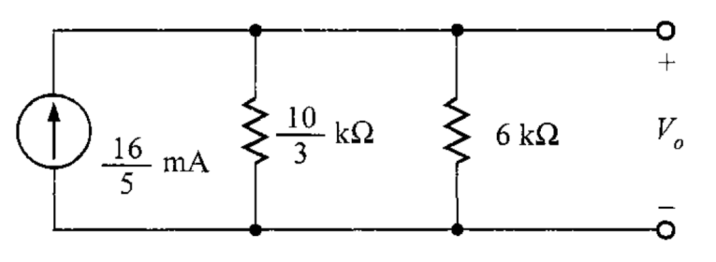
Figura 13. Conexión del circuito equivalente de Norton a la carga.

Finalmente, por ley de Ohm, se puede calcular el valor de $V_o$ , y es

$\displaystyle V_o = \left[\frac{\left(\frac{10}{3} \ \text{k} \right) \left(6 \ \text{k} \right)}{\frac{10}{3} \ \text{k} + 6 \ \text{k}} \right] \left(\frac{16}{5} \ \text{m} \right)$

$\displaystyle V_o = \left(\frac{20}{\frac{28}{3}} \ \text{k} \right) \left(\frac{16}{5} \ \text{m} \right) = \left(\frac{60}{28} \ \text{k} \right) \left(\frac{16}{5} \ \text{m} \right) = \left(\frac{15}{7} \ \text{k} \right) \left(\frac{16}{5} \ \text{m} \right)$

$\displaystyle V_o = \left(\frac{15}{7} \times 10^{3} \right) \left(\frac{16}{5} \times 10^{-3} \right) = \frac{48}{7}$

$\therefore \displaystyle V_o = \frac{48}{7}$

$\displaystyle (6 \ \text{k})I_1 - (2 \ \text{k}) I_2 = 6$	(1)
$\displaystyle I_2 = 2 \times 10^{-3}$	(2)

$\displaystyle (6 \ \text{k}) I_1 - (2 \ \text{k}) I_2 - (4 \ \text{k}) I_{sc} = 6$	(1)
$\displaystyle I_2 = 2 \times 10^{-3}$	(2)
$\displaystyle - (4 \ \text{k}) I_1 - (2 \ \text{k}) I_2 + (6 \ \text{k}) I_{sc} = 0$	(3)

$\displaystyle (6 \ \text{k}) I_1 - (4 \ \text{k}) I_{sc} = 10$	(4)
$\displaystyle - (4 \ \text{k}) I_1 + (6 \ \text{k}) I_{sc} = 4$	(5)

Teorema de Thévenin y de Norton para circuitos que incluyen únicamente fuentes independientes. Circuitos eléctricos.

Problemas resueltos

Primer método. Utilizando el teorema de Thévenin.

Segundo método. Utilizando el teorema de Norton.

Primer método. Utilizando el teorema de Thévenin.

Segundo método. Utilizando el teorema de Norton.

Publicado por Cesar Reyes

Deja un comentario Cancelar la respuesta

Teorema de Thévenin y de Norton para circuitos que incluyen únicamente fuentes independientes. Circuitos eléctricos.

Problemas resueltos

Primer método. Utilizando el teorema de Thévenin.

Segundo método. Utilizando el teorema de Norton.

Primer método. Utilizando el teorema de Thévenin.

Segundo método. Utilizando el teorema de Norton.

Comparte esto:

Relacionado

Publicado por Cesar Reyes

Deja un comentario Cancelar la respuesta