Fórmula de inversión compleja y el contorno de Bromwich. Laplace.

Introducción

Si $F(s) = \mathcal{L}[f(t)]$ , entonces $\mathcal{L}^{-1}[F(s)]$ está dada por

$\displaystyle f(t) = \frac{1}{2\pi i} \int_{\gamma - i \infty}^{\gamma + i \infty}{e^{st} \ F(s) \, ds}$ – – – (1)

donde $t>0$ y $f(t) = 0$ para $t<0$ . Este resultado se llama la inversión integral compleja o fórmula de inversión compleja. Tambipen se conoce como la fórmula integral de Bromwich. Este resultado ofrece un método directo para obtener la transformada inversa de Laplace de una función dada $F(s)$ .

La integración de la ecuación (1) se realiza a lo largo de un segmento $s=\gamma$ del plano complejo donde $s=x+iy$ . El número real $\gamma$ se escoge en tal forma que $s=\gamma$ quede a la derecha de todas las singularidades (polos, puntos de ramificación o singularidades escenciales); aparte de esta condición $\gamma$ es arbitraria.

Origen de la fórmula de inversión compleja

De acuerdo a la definición, se tiene que

$\displaystyle F(s) = \int_{0}^{\infty}{e^{-su} \ f(u) \, du}$

Entonces

$\displaystyle \lim_{T \rightarrow \infty}{\frac{1}{2\pi i} \int_{\gamma - iT}^{\gamma + iT}{e^{st} \ F(s) \, ds}} = \lim_{T \rightarrow \infty}{\frac{1}{2\pi i} \int_{\gamma - iT}^{\gamma + iT}{\int_{0}^{\infty}{e^{st - su} \ f(u) \, du} \, ds}}$

Asignando a $s=\gamma + iy$ y $ds = i \ dy$ , se transforma en

$\displaystyle \lim_{T \rightarrow \infty}{\frac{1}{2\pi i} \int_{\gamma - iT}^{\gamma + iT}{e^{st} \ F(s) \, ds}} = \lim_{T \rightarrow \infty}{\frac{1}{2\pi i} \int_{- T}^{T}{\int_{0}^{\infty}{e^{(\gamma + iy)t - (\gamma + iy)u} \ f(u) \, du} \cdot i \ dy}}$

$\displaystyle \lim_{T \rightarrow \infty}{\frac{1}{2\pi i} \int_{\gamma - iT}^{\gamma + iT}{e^{st} \ F(s) \, ds}} = \lim_{T \rightarrow \infty}{\frac{1}{2\pi} \int_{- T}^{T}{\int_{0}^{\infty}{e^{\gamma t} \ e^{i y t} \ e^{- \gamma u} \ e^{- i y u} \ f(u) \, du} \ dy}}$

$\displaystyle \lim_{T \rightarrow \infty}{\frac{1}{2\pi i} \int_{\gamma - iT}^{\gamma + iT}{e^{st} \ F(s) \, ds}} = \lim_{T \rightarrow \infty}{\frac{1}{2\pi} e^{\gamma t} \int_{-T}^{T}{e^{iyt} \, dy} \int_{0}^{\infty}{e^{- i y u} e^{- \gamma u} f(u) \, du}}$

$\displaystyle \frac{1}{2\pi i} \int_{\gamma - i \infty}^{\gamma + i \infty}{e^{st} \ F(s) \, ds} = \frac{1}{2\pi} e^{\gamma t} \int_{-\infty}^{\infty}{e^{iyt} \, dy} \int_{0}^{\infty}{e^{- i y u} [e^{- \gamma u} f(u)] \, du}$

$\displaystyle \frac{1}{2\pi i} \int_{\gamma - i \infty}^{\gamma + i \infty}{e^{st} \ F(s) \, ds} = \frac{1}{2\pi} e^{\gamma t} \left\{ \begin{matrix} 2\pi e^{-\gamma t} \ f(t) & t>0 \\ 0 & t<0 \end{matrix} \right.$

$\displaystyle \frac{1}{2\pi i} \int_{\gamma - i \infty}^{\gamma + i \infty}{e^{st} \ F(s) \, ds} = \left\{ \begin{matrix} \frac{1}{2\pi} e^{\gamma t} \cdot 2\pi e^{-\gamma t} \ f(t) & t>0 \\ \frac{1}{2\pi} e^{\gamma t} \cdot (0) & t<0 \end{matrix} \right.$

$\displaystyle \frac{1}{2\pi i} \int_{\gamma - i \infty}^{\gamma + i \infty}{e^{st} \ F(s) \, ds} = \left\{ \begin{matrix} f(t) & t>0 \\ 0 & t<0 \end{matrix} \right.$

por el teorema de la integral de Fourier. Así que

$\displaystyle \therefore f(t) = \frac{1}{2\pi i} \int_{\gamma - i\infty}^{\gamma + i\infty}{e^{st} \ F(s) \, ds}$ , $t>0$

como se esperaba.

En esta demostración se ha supuesto que $e^{-\gamma u} \ f(u)$ es absolutamente integrable en $(0, \infty)$ , es decir, que $\displaystyle \int_{0}^{\infty}{e^{-\gamma u} \ |f(u)| \, du}$ converge, para que sea lícito aplicar el teorema de la integral de Fourier. Para que está condición se cumpla es suficiente que $f(t)$ sea de orden exponencial $\gamma$ donde el número real $\gamma$ se escoge de tal manera que la recta del plano complejo $s=\gamma$ esté a la derecha de todas las singularidades de $F(s)$ . Aparte de esta condición, $\gamma$ se puede escoger arbitrariamente.

Contorno de Bromwich

En la práctica, la integral de la ecuación (1) se calcula mediante la integral curvilínea

$\displaystyle \frac{1}{2\pi i} \oint_{C}{e^{st} \ F(s) \, ds}$ – – – (2)

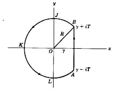
donde $C$ es el contorno de la figura 1. Este contorno, llamado contorno de Bromwich, se compone del segmento $AB$ y el arco $BJKLA$ de una circunferencia de radio $R$ con cento en el origen $O$ .

Si se representa el arco $BJKLA$ como $\Gamma$ , debido a que $T=\sqrt{R^2 - \gamma^2}$ (recordando el teorema de Pitágoras), la ecuación (1), se tiene que

$\displaystyle f(t) = \lim_{R \rightarrow \infty}{\frac{1}{2\pi i} \int_{\gamma - iT}^{\gamma + iT}{e^{st} \ F(s) \, ds}}$

$\displaystyle = \lim_{R \rightarrow \infty}{\left[ \frac{1}{2\pi i} \oint_{C}{e^{st} \ F(s) \, ds} - \frac{1}{2\pi i} \int_{\Gamma}{e^{st} \ F(s) \, ds} \right]}$ – – – (3)

Figura 7.1.1 Contorno de Bromwich — *Figura 1 Contorno de Bromwich.*

Estudio del contorno de Bromwich

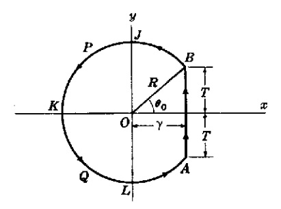
Sea $\Gamma$ la parte curva $BJPKQLA$ del contorno de Bromwich (figura 7.1.3) cuya ecuación es $s=Re^{i \theta}$ , $\theta_0 \le \theta \le 2\pi - \theta_0$ , es decir, el arco de una circunferencia de radio $R$ y centro en el origen. Se va a suponer que sobre $\Gamma$ se verifica que

$\displaystyle |F(s)| < \frac{M}{R^k}$

donde $k>0$ y $M$ son constantes.

Figura 7.1.3 Representando a Γ la parte curva BJPKQLA del contorno de Bromwich — *Figura 2, Representando a Γ la parte curva BJPKQLA del contorno de Bromwich*

Representando a $\Gamma_1$ , $\Gamma_2$ , $\Gamma_3$ y $\Gamma_4$ como los arcos $BJ$ , $JPK$ , $KQL$ y $LA$ , se tiene que

$\displaystyle \int_{BJPKQLA}{e^{st} F(s) \, ds} = \int_{BJ}{e^{st} F(s) \, ds} + \int_{JPK}{e^{st} F(s) \, ds} + \int_{KQL}{e^{st} F(s) \, ds} + \int_{LA}{e^{st} F(s) \, ds}$

$\displaystyle \int_{\Gamma}{e^{st} \ F(s) \, ds} = \int_{\Gamma_1}{e^{st} \ F(s) \, ds} + \int_{\Gamma_2}{e^{st} \ F(s) \, ds} + \int_{\Gamma_3}{e^{st} \ F(s) \, ds} + \int_{\Gamma_4}{e^{st} \ F(s) \, ds}$

Entonces, si se logra demostrar que cada una de las integrales del lado derecho tiende a cero cuando $R \rightarrow \infty$ , se habrá demostrado el resultado requerido. Así que, se resolverán cada una de las integrales:

$\displaystyle \lim_{R \rightarrow \infty}{\int_{\Gamma}{e^{st} \ F(s) \, ds}} = \lim_{R \rightarrow \infty}{\left[\int_{\Gamma_1}{e^{st} \ F(s) \, ds} + \int_{\Gamma_2}{e^{st} \ F(s) \, ds} + \int_{\Gamma_3}{e^{st} \ F(s) \, ds} + \int_{\Gamma_4}{e^{st} \ F(s) \, ds} \right]}$

$\displaystyle = \lim_{R \rightarrow \infty}{\int_{\Gamma_1}{e^{st} \ F(s) \, ds}} + \lim_{R \rightarrow \infty}{\int_{\Gamma_2}{e^{st} \ F(s) \, ds}} + \lim_{R \rightarrow \infty}{\int_{\Gamma_3}{e^{st} \ F(s) \, ds}} + \lim_{R \rightarrow \infty}{\int_{\Gamma_4}{e^{st} \ F(s) \, ds}}$

Análisis de la primera integral del miembro derecho.

$\displaystyle \int_{\Gamma_1}{e^{st} \ F(s) \, ds}$

Como $s = R e^{i \theta}$ , $ds = iR e^{i \theta} \ d\theta$ , $\theta_0 \le \theta \le \pi/2$ , se tiene a lo largo de $\Gamma_1$

$\displaystyle I_1 = \int_{\Gamma_1}{e^{st} \ F(s) \, ds} = \int_{\theta_0}^{\pi/2}{e^{R e^{i \theta} t} \ F(R e^{i \theta}) \cdot iRe^{i \theta} \, d\theta}$

$\displaystyle = \int_{\theta_0}^{\pi/2}{e^{R (\cos{\theta} + i \sin{\theta} ) t} \ F(R e^{i \theta}) \cdot iRe^{i \theta} \, d\theta} = \int_{\theta_0}^{\pi/2}{e^{(R \cos{\theta}) t} e^{i (R \sin{\theta}) t} \ F(R e^{i \theta}) \cdot iRe^{i \theta} \, d\theta}$

Entonces

$\displaystyle |I_1| \le \int_{\theta_0}^{\pi/2}{|e^{(R \cos{\theta}) t}| |e^{i (R \sin{\theta}) t}| \ |F(R e^{i \theta})| \cdot |iRe^{i \theta}| \, d\theta}$

$\displaystyle \le \int_{\theta_0}^{\pi/2}{e^{(R \cos{\theta}) t} \ |F(R e^{i \theta})| \cdot R \, d\theta}$

Tomando la condición dada $\displaystyle |F(s)| \le \frac{M}{R^k}$ (o mejor dicho, $\displaystyle |F(R e^{i \theta})| \le \frac{M}{R^k}$ ) sobre $\Gamma_1$

$\displaystyle |I_1| \le \int_{\theta_0}^{\pi/2}{e^{(R \cos{\theta}) t} \ \left( \frac{M}{R^k} \right) R \, d\theta} = \int_{\theta_0}^{\pi/2}{e^{(R \cos{\theta}) t} \ \left( \frac{M}{R^k} \right) \frac{1}{R^{-1}} \, d\theta}$

$\displaystyle = \frac{M}{R^{k-1}} \int_{\theta_0}^{\pi/2}{e^{(R \cos{\theta}) t} \, d\theta}$

Y tomando la transformación $\theta = \pi/2 - \phi$ [o mejor dicho $\displaystyle \theta_0 = \frac{\pi}{2} - \phi_0 = \arcsin{\left(\frac{\gamma}{R} \right)}$ ]

$\displaystyle |I_1| \le \frac{M}{R^{k-1}} \int_{\theta_0}^{\pi/2}{e^{(R \cos{\theta}) t} \, d\theta} \le \frac{M}{R^{k-1}} \int_{0}^{\phi_0}{e^{(R \sin{\theta}) t} \, d\phi}$

Ahora, como $\sin{\phi} \le \sin{\phi_0} \le \cos{\theta_0} = \gamma/R$ , resulta

$\displaystyle \large |I_1| \le \frac{M}{R^{k-1}} \int_{0}^{\phi_0}{e^{(R \sin{\theta}) t} \, d\phi} = \frac{M}{R^{k-1}} \int_{0}^{\phi_0}{e^{(R \cdot \frac{\gamma}{R}) t} \, d\phi}$

$\displaystyle = \frac{M}{R^{k-1}} \int_{0}^{\phi_0}{e^{ \gamma t} \, d\phi} = \frac{M}{R^{k-1}} e^{ \gamma t} \int_{0}^{\phi_0}{d\phi} = \frac{M}{R^{k-1}} e^{ \gamma t} (\phi_0 - 0)$

$\displaystyle = \frac{M}{R^{k-1}} e^{ \gamma t} \phi_0 = \frac{M}{R^{k-1}} e^{ \gamma t} \arcsin{\frac{\gamma}{R}}$

Por tanto, para la primera integral

$\displaystyle |I_1| \le \frac{M}{R^{k-1}} e^{ \gamma t} \arcsin{\frac{\gamma}{R}}$

$\displaystyle \lim_{R \rightarrow \infty}{|I_1|} \le \lim_{R \rightarrow \infty}{\left[\frac{M}{R^{k-1}} e^{ \gamma t} \arcsin{\frac{\gamma}{R}} \right]}$

$\displaystyle \lim_{R \rightarrow \infty}{\int_{\Gamma_1}{e^{st} \ F(s) \, ds}} \le \lim_{R \rightarrow \infty}{\left[\frac{M}{R^{k-1}} e^{ \gamma t} \arcsin{\frac{\gamma}{R}} \right]}$

$\displaystyle \lim_{R \rightarrow \infty}{\int_{\Gamma_1}{e^{st} \ F(s) \, ds}} = 0$

Análisis de la segunda integral del miembro derecho.

$\displaystyle \int_{\Gamma_2}{e^{st} \ F(s) \, ds}$

Como $s = R e^{i \theta}$ , $ds = iR e^{i \theta} \ d\theta$ , $\pi/2 \le \theta \le \pi$ , se tiene a lo largo de $\Gamma_2$

$\displaystyle I_2 = \int_{\Gamma_2}{e^{st} \ F(s) \, ds} = \int_{\pi/2}^{\pi}{e^{R e^{i \theta} t} \ F(R e^{i \theta}) \cdot iRe^{i \theta} \, d\theta}$

$\displaystyle = \int_{\pi/2}^{\pi}{e^{R (\cos{\theta} + i \sin{\theta} ) t} \ F(R e^{i \theta}) \cdot iRe^{i \theta} \, d\theta} = \int_{\pi/2}^{\pi}{e^{(R \cos{\theta}) t} e^{i (R \sin{\theta}) t} \ F(R e^{i \theta}) \cdot iRe^{i \theta} \, d\theta}$

Entonces

$\displaystyle |I_2| \le \int_{\pi/2}^{\pi}{|e^{(R \cos{\theta}) t}| |e^{i (R \sin{\theta}) t}| \ |F(R e^{i \theta})| \cdot |iRe^{i \theta}| \, d\theta}$

$\displaystyle \le \int_{\pi/2}^{\pi}{e^{(R \cos{\theta}) t} \ |F(R e^{i \theta})| \cdot R \, d\theta}$

Tomando la condición dada $\displaystyle |F(s)| \le \frac{M}{R^k}$ (o mejor dicho, $\displaystyle |F(R e^{i \theta})| \le \frac{M}{R^k}$ ) sobre $\Gamma_2$

$\displaystyle |I_2| \le \int_{\pi/2}^{\pi}{e^{(R \cos{\theta}) t} \ \left( \frac{M}{R^k} \right) R \, d\theta} \le \int_{\pi/2}^{\pi}{e^{(R \cos{\theta}) t} \ \left( \frac{M}{R^k} \right) \frac{1}{R^{-1}} \, d\theta}$

$\displaystyle = \frac{M}{R^{k-1}} \int_{\pi/2}^{\pi}{e^{(R \cos{\theta}) t} \, d\theta}$

Y tomando la transformación $\theta = \pi/2 + \phi$ [o mejor dicho $\displaystyle \theta_0 = \frac{\pi}{2} + \phi_0$ ]

$\displaystyle |I_2| \le \frac{M}{R^{k-1}} \int_{\pi/2}^{\pi}{e^{(R \cos{\theta}) t} \, d\theta} \le \frac{M}{R^{k-1}} \int_{0}^{\pi/2}{e^{-(R \sin{\phi}) t} \, d\phi}$

Ahora, como $\sin{\phi} \ge 2\phi/\pi$ para $0 \le \phi \le \pi/2$ , resulta

$\displaystyle \large |I_2| \le \frac{M}{R^{k-1}} \int_{0}^{\pi/2}{e^{-(R \sin{\phi}) t} \, d\phi} \le \frac{M}{R^{k-1}} \int_{0}^{\pi/2}{e^{-(R \cdot \frac{2\phi}{\pi}) t} \, d\phi}$

$\displaystyle = \frac{M}{R^{k-1}} \int_{0}^{\pi/2}{e^{-(\frac{2R \phi}{\pi}) t} \, d\phi} = \frac{M}{R^{k-1}} \cdot \left( - \frac{\pi}{2R t} \right) \left[e^{-(\frac{2R \cdot \frac{\pi}{2}}{\pi}) t} - 1 \right]$

$\displaystyle = - \frac{\pi M}{2tR^{k}} \left(e^{-R t} - 1 \right) = \frac{\pi M}{2tR^{k}} \left(1 - e^{-R t} \right)$

Por tanto, para la segunda integral

$\displaystyle |I_2| \le \frac{\pi M}{2tR^{k}} \left(1 - e^{-R t} \right)$

$\displaystyle \lim_{R \rightarrow \infty}{|I_2|} \le \lim_{R \rightarrow \infty}{\left[\frac{\pi M}{2tR^{k}} \left(1 - e^{-R t} \right) \right]}$

$\displaystyle \lim_{R \rightarrow \infty}{\int_{\Gamma_2}{e^{st} \ F(s) \, ds}} \le \lim_{R \rightarrow \infty}{\left[\frac{\pi M}{2tR^{k}} \left(1 - e^{-R t} \right) \right]}$

$\displaystyle \lim_{R \rightarrow \infty}{\int_{\Gamma_2}{e^{st} \ F(s) \, ds}} = 0$

De manera similar, para la tercera y cuarta integral

$\displaystyle \lim_{R \rightarrow \infty}{\int_{\Gamma_3}{e^{st} \ F(s) \, ds}} = 0$

$\displaystyle \lim_{R \rightarrow \infty}{\int_{\Gamma_4}{e^{st} \ F(s) \, ds}} = 0$

Finalmente

$\displaystyle \lim_{R \rightarrow \infty}{\int_{\Gamma}{e^{st} \ F(s) \, ds}} = \lim_{R \rightarrow \infty}{\int_{\Gamma_1}{e^{st} \ F(s) \, ds}} + \lim_{R \rightarrow \infty}{\int_{\Gamma_2}{e^{st} \ F(s) \, ds}} + \lim_{R \rightarrow \infty}{\int_{\Gamma_3}{e^{st} \ F(s) \, ds}} + \lim_{R \rightarrow \infty}{\int_{\Gamma_4}{e^{st} \ F(s) \, ds}}$

$\displaystyle \lim_{R \rightarrow \infty}{\int_{\Gamma}{e^{st} \ F(s) \, ds}} = 0 + 0 + 0 + 0$

$\displaystyle \lim_{R \rightarrow \infty}{\int_{\Gamma}{e^{st} \ F(s) \, ds}} = 0$

2 comentarios sobre “Fórmula de inversión compleja y el contorno de Bromwich. Laplace.”

Fernando dice:

11 enero, 2021 a las 3:08 pm

Seria tan amable de escribir mejor las formulas no es legible

Me gustaMe gusta

Responder
1. Cesar Augusto dice:
  
  13 enero, 2021 a las 12:22 pm
  
  Hola Fernando. Las fórmulas están legibles, el formato con el que estoy utilizando trata de adaptarlo al zoom y al tamaño de la ventana de el navegador. Algunas fórmulas son un poco extensas, por lo que es posible que se visualice un poco desordenado. Por el momento no realizo este tipo de situaciones.
  
  Me gustaMe gusta
  
  Responder